Exploratory Descision on Whisker Sensor to Maintain An Optimal Contact

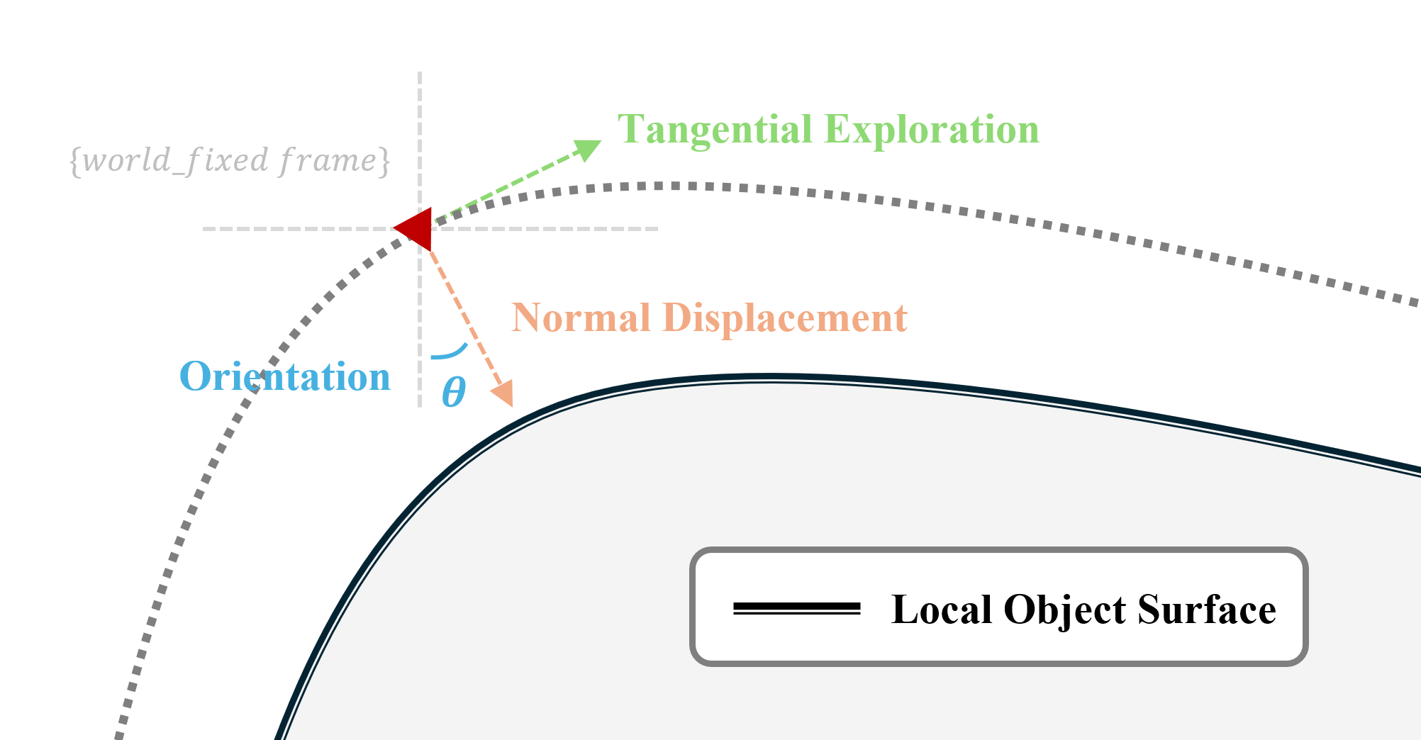
The tactile sensor explores around an object by maintaining its perceived orientation relative to surface feature or edge and moving tangentially (termed servoing) while tuning its normal displacement to ensure robust perception (termed active perception)

Basically, we intend to maintain a fixed optimal contact pose from whisker senor to obstacle surface, with proper contact height and orientation toward unknown surface. The detailed code demo is listed below in WhiskerActivePerception.py

Basic Design

---

Three general constraints were settled on the strategy:

• the end effector (whisker sensor) must move in a linear velocity with constant magnitude on world-fixed frame
• the forward trajectory of sensor must be paralleled with the reconstructed surface, the sensor was set to face right toward the object
• the normal displacement (distance or height) from sensor to contact surface must be a constant value

The last two constraints were used to maintain an optimal contact pose from sensor to surface and the target value were validate with multiple times in the off-line experiments on our calibration stage as in which the contact estimate was the most stable and accurate. The constant linear velocity magnitude is also important on two aspects: 1) transverse the dynamics on linear velocity of Y-axis to X-axis, the faster it goes on the Y represents a more significant change on the curvature of unknown surface, the slower it got on X-axis means we need to slow down the pace to adapt to the surface and get trustworthy estimates on tip position (which later we found is not true and totally unpractical in real world); 2) set fixed linear displacement between iteration and milestones, so as to give a quick extrapolate prediction on next contact according to the principle of Centripetal Parameterization along the fitted B-Spline.

Control Inputs

---

The control inputs on end-effector were separated into three basic elements:

• $\mid \vec{V_y^s} \mid$, the magnitude of linear velocity along the Y-axis of whisker-base frame
• $\mid \vec{V_x^s} \mid$, the magnitude of linear velocity along the X-axis of whisker-base frame
• $\theta$, an absolute target rotary position on world-fixed frame

which will later be transformed into the world-fixed frame.

Linear Velocity

I. Normal displacement

The linear velocity along the Y-axis of whisker base frame was used to keep track on the curvature of surface feature, along with the rotary control, to maintain a proper contact distance. The corrective component of this action moves the sensor radially towards a pre-set height relative to the edge. The direction is the same with the sensor orientation.

The contact distance is proportional to the whisker shaft’s deflection moment (or contact force), the closer to the surface the great it was deflected on the shaft and base device. So we use distance as a replacement but actually it is deflection moment that really matters. The deflection is controlled by a proportional-integral-derivative (PID) controller. A set point target, of magnetic field measurement on Y-axis from Hall effector sensor center, is determined after validation on varying contact distance by our 2D motorized stage.

The detailed implementation is as followed:

class PIDController:
    def __init__(self, Kp, Ki, Kd, set_point=0) -> None:
        self.Kp = Kp
        self.Ki = Ki
        self.Kd = Kd
        self.set_point = set_point
        self.previous_error = 0
        self.integral = 0
        self.previous_time = rospy.get_time()

    def update(self, measured_value):
        current_time = rospy.get_time()
        dt = current_time - self.previous_time
        if dt <= 0.0:
            dt = 1e-6  # Avoid division by zero or negative time intervals

        error = np.abs(measured_value) - np.abs(self.set_point)
        self.integral += error * dt
        derivative = (error - self.previous_error) / dt

        output = self.Kp * error + self.Ki * self.integral + self.Kd * derivative
        self.previous_error = error
        self.previous_time = current_time
        
        return -output

Be careful about the output direction here. Adjustment should be made according to the target deflection (plus or minus) you set.

II. Tangential exploration

We were originally thinking a dynamic constraint on tangential movement would benefit it by slowing down the pace on sharp curvature surface, but it turns out would cause even more trouble on our active reconstruction. A misbalance between tangential movement and normal displacement results in an axial slip along the whisker shaft from time to time (you need actually somewhat speed up when approaching the surface on radial direction, pushing the shaft against the edge without a forward movement to compensate it would definitely ends up with an axial slip). Therefore in the real experiment, I set a prefixed tangential displacement on the trajectory.

Rotary Control

I. B-Spline Curve fitness

• Closeness: Difference between splrep and splprep , apparently there’s a better fit on 1D-curve where $y = f(x)$ using splrep. Yet in our application scene, the contact state is on a 2D coordinate with no correlation in dimensions. So I have to use the splprep

• Smoothness: I’m relying on the needed knots and quantile to adjust the trade-off between the smoothness and closeness. It could always give a relatively promising result automatically. Smooth condition seems always asks a manually regulation according to the number of data points if we used a s parameter.

    # knots quantile
    n_interior_knots = 2
    qs = np.linspace(0, 1, n_interior_knots+2)[1:-1]
    knots = np.quantile(x, qs)
    tck_q, u = interpolate.splprep([x, y], t=knots, k=3)
  

II. Implementation Details

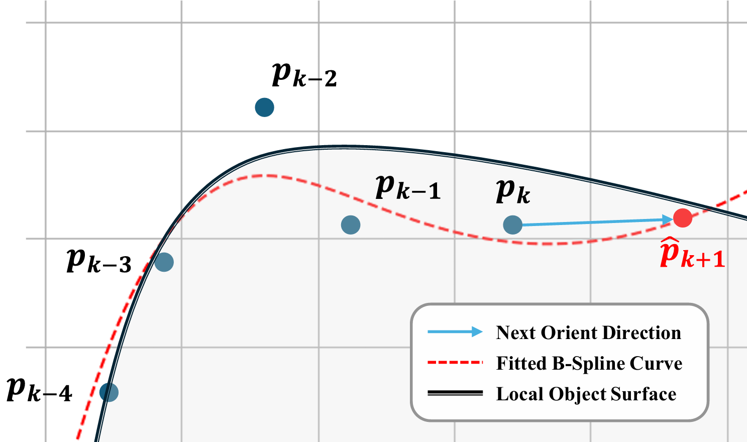
Fig. 4. Prediction on next contact point using B-Spline curve and $N$ previous key reconstructs \(\left \{ \boldsymbol{p}_{k-i} \mid i=0, 1,...,n-1 \right \}\). The slope between current contact point \(\boldsymbol{p}_{k}\) and next prediction \(\hat{\boldsymbol{p}}_{k+1}\) is regards as the next orient direction.

# Extrapolate distance for iterations
u_next = 1 + 1 / (keypoint_length - 1)

if touch_index % keypoint_interval == 0:
	# A deque is maintained for previous key points
  keypoints_deq.append(tip_pos_w_filtered_que[-1])

  if len(keypoints_deq) == keypoint_length:
      # Predict next contact position along BSpline curve
      qs = np.linspace(0, 1, n_interior_knots + 2)[1:-1]
      knots = np.quantile(np.array(keypoints_deq)[:,1], qs)
      tck, u = interpolate.splprep(
          [np.array(keypoints_deq)[:,0],
          np.array(keypoints_deq)[:,1]],
          t=knots,
          k=spline_degree,
      )
      tip_pos_w_next = interpolate.splev(u_next, tck)
      # Transform a slope to next contact into angular measurement
      theta_next_measured = np.arctan2(
          tip_pos_w_next[1] - np.array(keypoints_deq)[-1][1],
          tip_pos_w_next[0] - np.array(keypoints_deq)[-1][0])
      # Refine the orientation target
      theta_next_desired = refineOrientation(theta_next_measured)

• B-Spline curve is built from $N$ previous key points, to extract the local curvature from surface and predict the next contact position \(\hat{\boldsymbol{p}}_{k+1}\). The splprep function in the scipy.interpolate module by default uses centripetal parameterization. This method helps to prevent clustering of parameter values, which can lead to better and more stable spline fitting, especially for datasets where points are not uniformly spaced.
• The slope from current contact \(\hat{\boldsymbol{p}}_k\) to next prediction \(\hat{\boldsymbol{p}}_{k+1}\) is transformed to angular rotation as the target orientation for next iteration. This calculation is further refined later in refineOrientation function, to process the wrap from a whole round and apply a rotary speed limitation, making sure it match for the Franka robot coordinate.
• A distance of 5 general works fine in real experiment for the interval between sampled key points. They still overlaps from each other occasionally due to the fluctuation, even though after the Bayesian filter. The keypoint_length and keypoint_interval influence the sensitivity of rotary decision on curved contour.
• $u_{next}=1 + 1 / (KeypointLength - 1)$ as centripetal parameter value, is used to extrapolate the next prediction. Firstly, the sampling rate is quite fast of 300Hz, the actual displacement between iterations is relatively small therefore ignorable. Moreover, we hold a constant tangential velocity. To recap, the iterative distance is generally equal.

III. About Refinement

Wrap detection after a whole round and transform the angular target according to the robot frame.

# detect wrap 
if r > 0 and theta_last_measured < 0 : # -pi -> pi & +0 -> -0 : clockwise : we were forwarding along this direction, so increase wrap in this block
  wrap_count += 1
elif r < 0 and theta_last_measured > 0 : # pi -> -pi & -0 -> +0 : counter clockwise
  wrap_count -= 1
r_refined = r - wrap_count * 2 * np.pi

Smooth the rotary transition by limit the speed on different direction.

if touch_index >= stable_distance:
  rot_speed_limit = rot_limit_scale * keypoint_interval # Multiply a servoing ratio (keypoint_interval) to regulate our limit
  theta_err = r_refined - theta_last_desired
  
  if (theta_err > rot_speed_limit * 0.2 and theta_err < 0.5 * np.pi) or \
    (theta_err < - 1.5*np.pi and theta_err > - 2*np.pi + rot_speed_limit *0.2) or \
    (theta_err <= -0.5*np.pi and theta_err >= -np.pi) or \
    (theta_err >= np.pi and theta_err <= 1.5*np.pi):
    r_refined = theta_last_desired + rot_speed_limit * 0.6 # Convex object, so generally only need a rotation toward one direction
	elif (theta_err < -rot_speed_limit and theta_err > -0.5 * np.pi) or \
    (theta_err > 1.5*np.pi and theta_err < 2*np.pi - rot_speed_limit) or \
    (theta_err >= 0.5*np.pi and theta_err <= np.pi) or \
    (theta_err <= - np.pi and theta_err >= - 1.5*np.pi):
    r_refined = theta_last_desired - rot_speed_limit 

Finally, all the desired control commands would be sent to robot_control node to drive the Franka robot in real-time based on the contact information from whisker sensor.