Filter the Tip Estimates Based on An Assumption of Relative Static Contact

Objective

---

Visualizing the whole reconstruction on tip position in a experiment of 2D plane straight surface, the results were clearly separated by two different phase, as it could be seen from the Figure 1. :

• the contacts were on the whisker’s shaft, where the friction is more stable thus the less fluctuation on whisker’s deflection state, that is to say, the tip position estimates were also smoother;
• the contacts were on the whisker’s tip, the friction on contact point was heavily affected by the texture, force magnitude and direction, thus an unstable reconstruction on tip position.

Fig. 1-A Tip position under whisker-base frame; B Tip position under world-fixed frame with constant linear displacement along X-axis

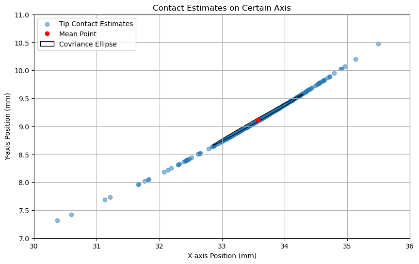
Another fact is that the tips (or contact position, if it was touched by the tip point of whisker shaft), even though unstable, were still dancing around the curve profile of the whisker’s tip path. And since the x position and y position were bother calculated from a same deflection moment by different characterized polynomial model, they were correlated, thus obey specific co-variance distribution under certain optimal deflection state, with fixed contact height and sensor orientation toward obstacle, as it was showed in the underneath figure.

Fig.2 Estimates distribution within tip contact phase

We have to reduce the noise of the direct tip estimates from our previous method, otherwise the reconstruction would be intolerantly unstable and cause problem on our next tactile servoing task, of which calculating the forward direction for next moment is essential (Fig. Slope of fitted lines from N consecutive points were quite unstable).

Bayesian Filter

---

Given the first and the most important hypothesis here: the whisker shaft would maintain its optimal deflection state, that is to say, a fixed contact height and parallel orientation from object surface, based on our automatic control strategies and thus the tip position would be static. To recap:

\[\hat{X}_{k}^-=\hat{X}_{k-1}\]

$X_{k}$ is the state variable of $k$ iteration which represent of a 2-dim coordinate position for tip point under whisker-base frame. Since our filtering target is the direct output from our previous tip estimate method, the measurement $Z_{k}$ would also be a 2-dim coordinate. Under a same frame and with same physical representation, the transform matrix $H$ would be a simple eye matrix, so was the state transition matrix $F$ according to the hypothesis equation upon.

# Initialize the kalman filter

kf = KalmanFilter(dim_x=2, dim_z=2)
kf.x = np.array([33.6, 9.1])   # 2d coordinates on X- and Y-axis, z was the position directly measured on two dimensions
kf.F = np.array([[1., 0.], [0., 1.]])
kf.H = np.array([[1., 0.], [0., 1.]])
kf.P *= 10.
kf.R = np.eye(kf.dim_z)
kf.Q = np.eye(kf.dim_x)*0.01

The Kalman filter calculates the optimal state of each uncorrelated tip position by weighting the previous state (predict step) and the predicted noisy tip point by our characterized polynomial model (measurement step):

\[\begin{equation}\begin{array}{ll}\mathit{Predict \ Step} & \quad \mathit{Measurement \ Update} \\\hat{x}_k^- = \hat{x}_{k-1} & \quad K_k = P_k^- (P_k^- + R_k)^{-1} \\P_k^- = P_{k-1} + Q & \quad \hat{x}_k = \hat{x}_k^- + K_k (z_k - \hat{x}_k^-) \\& \quad P_k = (1 - K_k) P_k^-\end{array}\end{equation}\]

The measurement noise was updated empirically for every iteration based on 5 consecutive estimated point from polynomial model. Extract 5 points and calculate their co-variance matrix as the measurement noise $R_{k}$ for current iteration.

# Interatively updated measurement and process noise
def update_noise_matrices(kf, measurements):
    # The measurement noise R - covariance matrix was determined and updated empicically by the most recently collected data points
    # sampled length : window_size = 5, including the value on current index

    zset = np.array(measurements)
    kf.R = np.cov(zset[:, 0], zset[:, 1])
    
    # ...

The process noise $Q$ was set to be constant, an eye matrix multiplied by 0.01 as confidence for our transition hypothesis and tactile servoing strategy. I’m actually intend to make it adaptable at the first place, based on the control dynamic as a measurement about how I trust the constant state assumption yet haven’t found a suitable approach. Moreover, the current setting on $Q$ can not reflect the correlation between the X and Y, therefore after filtering the post distribution was more concentrated yet a bit out of the curve profile of whisker’s detach line.

for index, z in enumerate(measurements):
    if index < 5: continue
    update_noise_matrices(kf, measurements[(index+1-window_size):index+1])  # DYX: remember to deal with the edge members
    kf.predict()
    kf.update(z)
    uxs.append(kf.x.copy())

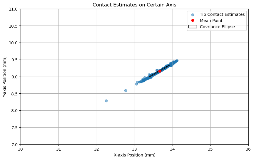
Fig. Distribution after filtering

$Cov Matrix: \newline \begin{bmatrix} 0.517804&0.327320&0.327320&0.20787 \end{bmatrix}\to \begin{bmatrix} 0.078676&0.050925&.050925&0.033202 \end{bmatrix}$

The uncertainty of model worth to be further explored in the future.