Building Filter Block and Test on Offline Data from Whisker Sensor

Problem Statement

---

2D contact position inference for whisker sensor. The basic format of state estimation equation is showed as follows:

\[x_{k+1}=\mathbf{A}x_{k}+\mathbf{B}\begin{bmatrix}v_{sb}^{b}\\w_{sb}^{b}\end{bmatrix}+w_{k} \\ y_{k}=g(x_{k})+v_{k}\]

The problem was under 2D scene therefore the contact point was descripted by a 2-dimensional vector and the most important hypothesis made here was that, the contact was always static that is to say the position was fixed under world reference frame.

• State Variable (where $z=0$ in 2d scene)

\[\mathit{\mathbf{x}} = [x, y, z]\]

Process Model

---

• State Transition and System Input

Back to problem description, $v_{sb}^b$ and $w_{sb}^b$ are the linear and angular velocity respectively, of sensor base \(\left \{ B \right \}\) relative to world-fixed frame \(\left \{ S \right \}\) as viewed in the body frame. $x_k=p_c$ is the position vector of the contact point relative to origin of \(\left \{ B \right \}\) at time-step $k$. We can first calculate the linear velocity of $p_c$ with respected to world frame:

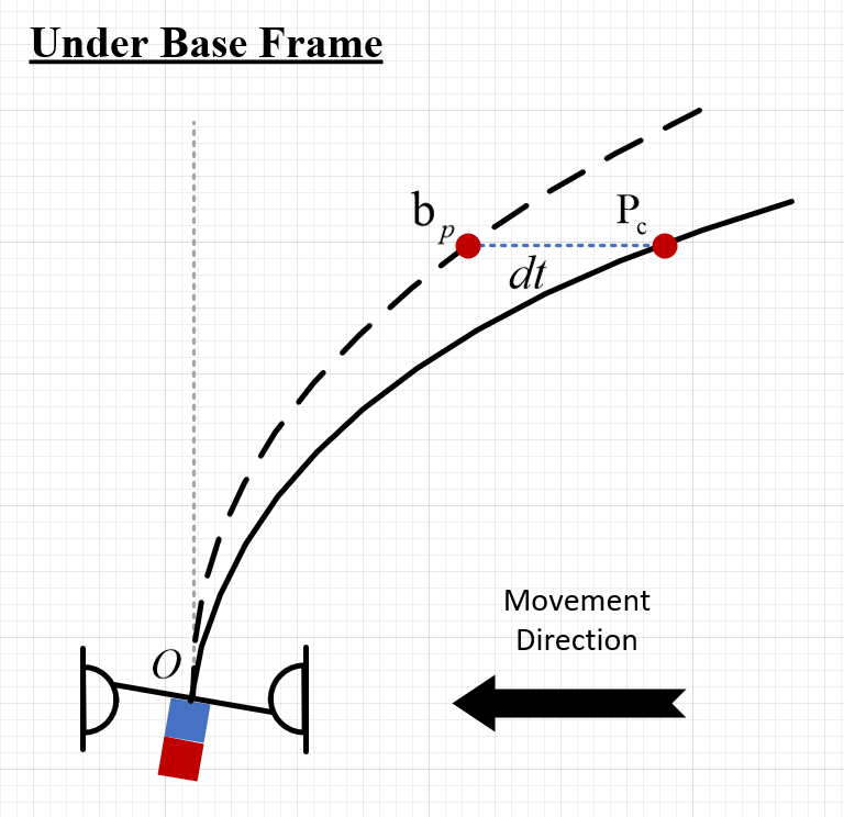
\[v_{sp_c}^b=v_{sb_p}^b+v_{bp_c}^b=v_{sb}^b+w_{sb}^b\times b_p+v_{bp_c}^b\]

Define a point $b_p$ that is instantaneously coincident to $p_c$ but fixed in \(\left \{ B \right \}\) . The movement of contact under world frame was actually divided into two part: 1) the constant whisker base movement which correspond to the movement of fixed point $b_p$ 2) and the contact shift under base frame $v_{bp_c}^b$ after a nominal short time interval $dt$.

Given the hypothesis we made at the very begin, the contact was always static in the world frame, thus there’s $v_{sp_c}^b=0$ ( or say $v_{bp_c}^b=-v_{sb_p}^b$, there’s another perspective to under this problem, we can conclude that the moving distance for $b_p$ in \(\left \{ S \right \}\) equals to it for $p_c$ in \(\left \{ B \right \}\) within a nominal short time deviation $dt$). And we can calculate the $v_{bp_c}^b$ as follows:

\[\begin{equation}v_{bp_c}^b=-v_{sb}^b+-w_{sb}^b\times b_p = -\begin{bmatrix} \mathbf{I} & -\left [ \mathbf{p_c} \right ] \end{bmatrix}\begin{bmatrix} v_{sb}^b \\ w_{sb}^b \end{bmatrix}\end{equation}\]

The process model can expressed as

\[x_{k+1}=x_k+\delta_tv_{bp_c}^b=x_k-\delta_t \begin{bmatrix} \mathbf{I} & -\left [ \mathbf{p_c} \right ] \end{bmatrix}\xi_{sb}^b+w_k\]

which gives $\mathbf{A}=\mathbf{I}$ and $\mathbf{B}=-\delta_t \begin{bmatrix} \mathbf{I} & \left [ \mathbf{p_c} \right ] \end{bmatrix}$.

❓ It is of vital importance to understand what exactly happened in equation (1), yet there seems to be some mistake of the formulation in original paper. I’m not totally sure. There’s should be a minus before the skew-symmetric matrix of $p_c$, to set the cross product in order:

\[-w_{sb}^b \times b_p = b_p \times w_{sb}^b = \left [ p_c \right ]w_{sb}^b\]

But there’s none in the paper, I have to make sure who’s right here…

To implement it as a state transition function in Kalman Filter:

v_bpc_b = -v_sb_b + -np.cross(w_sb_b, bp ) # direct corss product 

def f_contact(x, lv, av, dt):
    input = np.append(lv, av, axis=0)
    B = -dt*np.append(np.identity(3), -skew(x), axis=1)
    A = np.identity(3)
    prior_predict = A @ x + B @ input 
    return prior_predict

The function will return prior prediction without process noise for later operation.

BTW, we could calculate the contact point velocity $v_{bp_c}^b$ either by direct cross product according to the front part of (1) or in a totally matrix multiplication manner which could save the computation cost.

• Process Noise

Q = np.array([[.001, 0, 0], [0, .001, 0], [0, 0, .00001]])

$z$ always equals to zero in 2d scene, therefore I set the variance on z-dimension to be $1e^{-5}$. It is reasonable since $z$ value never change in our system. And the x- and y- variance to be relatively larger yet considerable. Meanwhile, as coordinate vector, there’s no relation between three variables thus this covariance matrix was set to be zero except the diagonal.

Measurement Model

---

• Data Collection

Whisker base and world frame coordinate

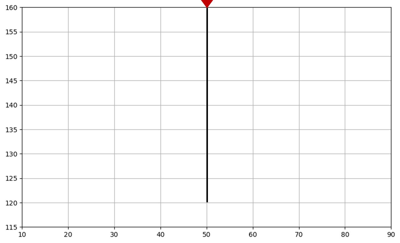
5 per step on X- and Y- axis, from 10 to 90 and 115 to 160 respectively. 170 sets of magnetic data which contains 9 sequential magnetic readings on three dimensions within fixed static period were collected in all. Average value was calculated on both side and also the middle column (which was collected two times when sampling and moving touch rod from both side, and the average value was extract from both sets)

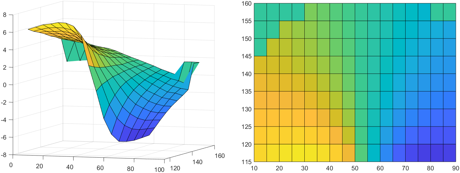
Sampling data on Y-axis of magnetic readings, 3D and 2D format (the coordinate on y-axis was upside-down, be careful, I haven’t fixed it!)

The reading on Y-axis is most significant, the variance is much bigger comparing with other two dimension.

☝🏼 We shall try to analysis this result according to the physically reality:

1. The surface on left and right upper corner collapse, it probably because the whisker body has detached from the rigid touch rod. The contact range has been surpassed.
2. A significant convex curve can be noticed on both side near the whisker base line, where $y$ approximately near 160. It is because the touch rod now, has been really closed to the whisker base, the whisker body was in its maximum deflection presently. Thus a bounce-back is reasonable considering a low fraction force along whisker and its own resilience.

• Bivariate Polynomial Model

The previously mentioned data were imported into a custom polynomial model to fit and build the measurement model. A multi-order polynomial model on 3d scene was built based on numpy.linalg.lstsq, to fit $f(x, y)=z$. Most python package only provide 2d implementation, like numpy.polyfit. Discussion here is quite helpful.

def polyfit2d(x, y, z, kx=5, ky=5, order=None):
    """
    Two dimensional polynomial fitting by least squares.
    Fits the functional form f(x,y) = z.

    Notes
    -----
    Resultant fit can be plotted with:
    np.polynomial.polynomial.polygrid2d(x, y, soln.reshape((kx+1, ky+1)))

    Parameters
    ----------
    x, y: array-like, 1d
        x and y coordinates.
    z: np.ndarray, 2d
        Surface to fit.
    kx, ky: int, default is 3
        Polynomial order in x and y, respectively.
    order: int or None, default is None
        If None, all coefficients up to maxiumum kx, ky, ie. up to and including x^kx*y^ky, are considered.
        If int, coefficients up to a maximum of kx+ky <= order are considered.

    Returns
    -------
    Return paramters from np.linalg.lstsq.

    soln: np.ndarray
        Array of polynomial coefficients.
    residuals: np.ndarray
    rank: int
    s: np.ndarray

    """

    # grid coords
    x, y = np.meshgrid(x, y)
    # coefficient array, up to x^kx, y^ky
    coeffs = np.ones((kx + 1, ky + 1))

    # solve array
    a = np.zeros((coeffs.size, x.size))

    # for each coefficient produce array x^i, y^j
    for index, (i, j) in enumerate(np.ndindex(coeffs.shape)):
        # do not include powers greater than order
        if order is not None and i + j > order:
            arr = np.zeros_like(x)
        else:
            arr = coeffs[i, j] * x**i * y**j
        a[index] = arr.ravel()

    # do leastsq fitting and return leastsq result
    print(a.T.shape, np.ravel(z).shape)
    return np.linalg.lstsq(a.T, np.ravel(z), rcond=None)

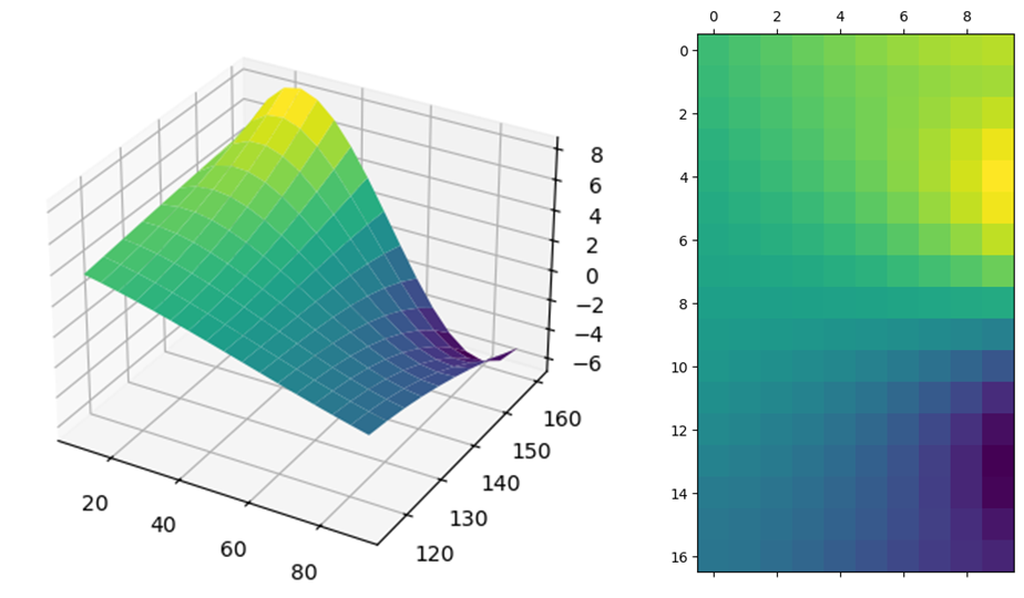
Polynomial model fitted surface, 3D and 2D format

Polynomial regression for whisker data resulted in R-squared value of 0.99442 and Root-Mean Squared Error (RMSE) of 0.23193.

• Measurement Model and Noise

The sensor noise variance was chosen to be 0.0537 (0.23193**2) which was found through RMSE of the calibration results of measurement model reported previously.

def h_contact(x):
		# polynomial.polyval2d should be alright
    return np.polynomial.polynomial.polygrid2d(x[0], x[1], coeff.reshape((6, 6)))

R = np.array([[rms**2]]) # Measurement Noise

Filter Implementation

---

• Synthesized Data

Prepare trajectory, corresponding magnetic data and also fictitious linear & angular velocity:

# Corresponding linear and angular velocity
linear_vel = np.array([.5, .125, 0])
angular_vel = np.array([0, 0, 0])
u = np.append(linear_vel, angular_vel, axis=0)

# Magnetic data on Y axis generated from measurement model according to the start point and end point of test trajectory
trajecotry_ = np.polynomial.polynomial.polyval2d(
    np.linspace(X_start, X_end, 160),
    np.linspace(Y_start, Y_end, 160),
    coeff.reshape((6, 6)),
)
zs = [np.array([trajecotry_[i]]) for i in range(trajecotry_.shape[0])]

• Unscented Kalman Filter Test

Time interval $dt$ was set to be 1.0. Instantiate the UKF:

sigmas = MerweScaledSigmaPoints(3, alpha=.1, beta=2., kappa=0.)
ukf = UKF(dim_x=3, dim_z=1, fx=f_contact,
          hx=h_contact, dt=dt, points=sigmas)

Estimated trajectory from [10, 125] straight to [90, 145] and ground truth

Bayesian Filter UKF tracked on ground truth with a lowest Euclidean Distance of 0.311 millimeters and with a standard deviation of 0.801 millimeters. And it costs 68 steps to converge to within 1mm of true location.

⛔ There’s probably an unsolved issue in the unscented transform function of filterpy package (Version 1.4.5). In the update function of UKF Implementation, remember to reshape the sigmas point matrix with: self.sigmas_h = np.atleast_2d(sigmas_h).reshape((-1, 1)) # DYX: reshape , before send it into the transform function. The original irregulated array can’t be directly dot multiply to the weight matrix in UT.

Different initial position for a same ground truth trajectory, [10, 125]~[90, 145]

There were a noticeable bounce near the middle, where $x \rightarrow 50$. It probably results from our sampling data of middle column when contact the whisker from both sides. We shall try to resolve this problem later.

Future Improvement

---

• Contact along surface - dynamic contact solution

  Back to the hypothesis we have made at very begin, “the contact was always static”. Presume there’re two types of contact in the real world: 1) contact by a rigid touch rod; 2) contact by real object along its surface and whisker length. In the former situation, it is easy to imagine that the contact position, which attached on the rigid rod, is always fixed in the world frame. Of course it is since the rod would never move, only the whisker itself. However as for the latter situation, the contact will continue to shift along the surface with a dynamic position in world frame. Therefore the process model would fail here.

  To compensate that, with no applicable modeling for that part of state transition, we can either 1) introduce an extra fictitious process noise in the model; 2) or conduct fading memory (FM) in the calculation of estimation error covariance:

  \[\tilde{\mathbf{P}} = \alpha^2\mathbf{FPF^\top}+\mathbf{Q}\]

  Neither of these two approach bear a great confidence on prior prediction thus decrease its proportion on the data fusion in different manner. By conduct a scale factor $\alpha$, thus it spare greater weight on the more recent measurements, and forget the history estimation (that is to say, “fading memory”).

    filter.Q = Q_discrete_white_noise(dim=2, dt=dt, var=20.) # increase process noise
    filter.alpha = 1.00 # scaling factor of FM
  

  Both of which were built in the implementation of Kalman Filter in filterpy.

• Introduce magnetic readings of multi-dimension

  I only include the magnetic readings on Y axis as the $z$ measurement. The X- and Z-axial reading should also be introduced into the model later, moreover, a covariance between variables (physically they were correlated in reality with a prior mathematical model) may further improve the model?