Details of Bayesian Filter and Kalman Gain - Vol.1
Introduction
1. Recursive Algorithm
Let’s introduce the concept by a simple example.
Presuming there’s a long rigid rod with unknown length $X$. We want to get a optimal prediction $\hat{X}$ on its length with an inaccurate measurement device (let’s pretend our ruler is really that bad…). Intuitively, the most accurate prediction comes from an average of multiple-times of measurement $Z_{k}$, where $k$ represents the index for different measurement:
\[\begin{align*} \hat{X}_k =& \frac{1}{k}(Z_1+Z_2+...+Z_k) \\ =& \frac{1}{k}(Z_1+Z_2+...+Z_{k-1})+\frac{1}{k}Z_k \\ =& \frac{1}{k} \cdot \frac{k-1}{k-1} \cdot (Z_1+Z_2+...+Z_{k-1})+\frac{1}{k}Z_k \\ =& \frac{k-1}{k} \cdot \hat{X}_{k-1}+\frac{1}{k}Z_k \\ =& \hat{X}_{k-1}+\frac{1}{k}(Z_k-\hat{X}_{k-1}) \end{align*}\]The $\frac{1}{k}$ exactly represent a kind of Kalman Gain $K_k$ here in $k~th$, . The equation above can be interpret as :
\[Current Estimation = Last Estimation + K_k \times(Current Measurement - Last Estimation)\]Come back to our topic, Kalman Filter is a kind of optimal recursive data processing algorithm. What recursive means here in this example, is the iterative prediction based on all the former estimation which typically is the truth when introduce it into the sequential state estimation problem of any dynamic system, either it is continuous or discrete. But of course in a totally different format.
Let’s replace the Kalman Gain here with:
\[K_k=\frac{e_{EST_{k-1}}}{e_{EST_{k-1}}+e_{MEA_{k}}}\]where $e_{EST}$ and $e_{MEA}$ represent the estimation error and measurement error. Let’s see what will happened:
\[\begin{align*} & when \quad e_{EST_{k-1}} >> e_{MEA_{k}}, \quad K_k \to 1 \Rightarrow \hat{X}_k = \hat{X}_{k-1}+Z_k-\hat{X}_{k-1} = Z_k \\ & when \quad e_{EST_{k-1}} >> e_{MEA_{k}}, \quad K_k \to 0 \Rightarrow \hat{X}_k = \hat{X}_{k-1}+0 \cdot (Z_k-\hat{X}_{k-1}) = \hat{X}_{k-1} \end{align*}\]This fit our intuition. If our previous prediction is so unpromising, we will lean more on current measurement, vice versa, if the ruler’s measurement results were too unstable, we will take our previous prediction in history into more consideration. It seems to be very reasonable, and actually fits the basic format of Kalman gain in state estimation problem for linear discrete dynamic system.
2. State Estimation
We have a bad estimation $\hat{X}$ (which comes from last prediction, system input and an analytical model with unpredictable noise) and a bad measurement $Z$ (which comes from sensor sampling data with noise and a measurement model) that suffer from an uncertainty in the real world, and we want to fuse these two results to produce an optimal prediction, where the Kalman Filter therefore be introduced. And to calculate the Kalman Gain $K_k$ on every iteration is of vital importance in this algorithm.
State transition and measurement model
\[\left\{\begin{matrix} & X_k = AX_{k-1} + B\mu_{k-1} + \omega_{k-1} \quad & \mu \sim \aleph(0, Q)\\ & Z_k = HX_k + \upsilon_{k} \quad & \upsilon \sim \aleph(0, R) \end{matrix}\right.\]
We will back here later with details and reveal the whole objectives of this log, that is the calculation of the Kalman gain in state estimation of linear discrete dynamic system.
By the way, the uncertainty here comes from two different aspect:
- No perfect mathematical analytical model to describe a dynamic system to produce direct estimation. In this example, our estimation comes from all previous measurements, but in most other cases, an analytical model will be built independent from measurement what we call ‘process model’ or ‘state transition model’.
- No perfect sensor or impossible to directly measure. All the sensor suffers from a noise, moreover, sometimes, we even can’t directly collect the measurement. For example, rocket engineer want to know the inner temperature of tunnel engine yet no sensor could survive from that. Thus a sensor attached outside the engine tunnel will be applied and an indirect measurement, which suffers from a even more severe noise, will be combined with analytical model of this dynamic system to make prediction.
Be prepare to calculate the Kalman Gain
1. Data Fusion
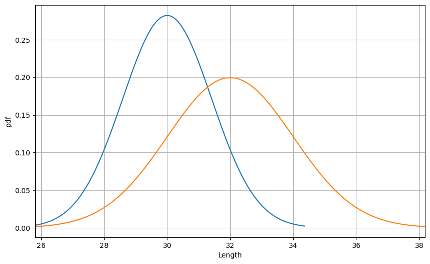
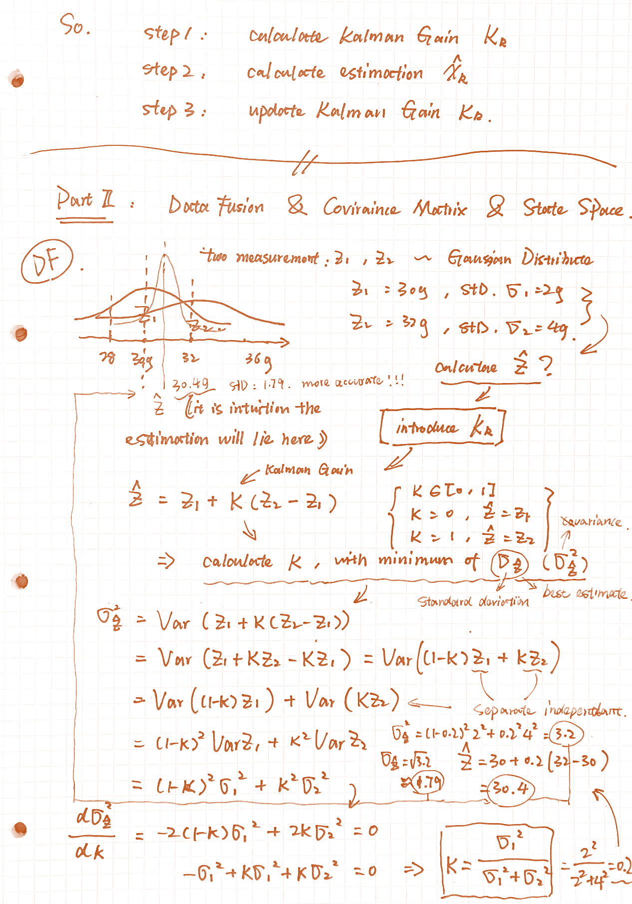
Assuming there were two different rulers which give us two different sets of measurement results, $Z_1$, $Z_2$, both of the results are uncertain and in gaussian distribution:
\[\begin{align*} & Z_1 : mean=30, variance=2 \\ & Z_2 : mean=32, variance=4 \end{align*}\]Making a prediction on where the optimal estimation result $\hat{Z}$ may lie, we probably think it was in between two peaks and closer to the $Z_1$. Since it bears a lower variance which means it has a less significant noise and has a better measurement.
 Fig 1. Two sets of measurement results which were in gaussian distribution.
Let introduce the concept of data fusion here by including the Kalman gain into our estimation:
\[\hat{Z} = Z_1 + K(Z_2 - Z_1)\]Our best prediction comes from the fusion of two bad measurements, and of course it is with a lowest variance, or covariance. So we need to calculate out a gain factor $K$ to make it possible.
\[\begin{align*} \sigma_{\hat{Z}}^2 &= Var(Z_1+K(Z_2-Z_1)) \\ &= Var((1-K)Z_1+KZ_2) \\ \end{align*}\]where $Z_1$ and $Z_2$ are two separately independent variables, thus:
\[\begin{align*} \Rightarrow \sigma_{\hat{Z}}^2 &= Var((1-k)Z_1) + Var(KZ_2) \\ &= (1-K)^2Var(Z_1) + K^2Var(Z_2) \\ &= (1-K)^2 \sigma_1^2 + K^2 \sigma_2^2 \end{align*}\]calculate its derivatives on $K$ to find the minimum point:
\[\begin{align*} \frac{d\sigma_{\hat{Z}}^2}{dK} = -2(1-K)\sigma_1^2 + 2K\sigma_2^2 &= 0 \\ -\sigma_1^2 + K\sigma_1^2 + K\sigma_2^2 &= 0 \\ \Rightarrow K &= \frac{\sigma_1^2}{\sigma_1^2 + \sigma_2^2} \end{align*}\]where $\sigma_1$ equals to $2$ and $\sigma_2$ equals to $4$ in our example,
\[K=\frac{2^2}{2^2+4^2}=0.2 \Rightarrow \hat{Z}=30+0.2(32-30)=30.4\]It gives us a best estimation of $30.4$, and the variance is of $1.79$ which is lower than both of $Z_1$ and $Z_2$. So as our story telling, fuse two bad prediction to give a better estimation with costumed Kalman gain.
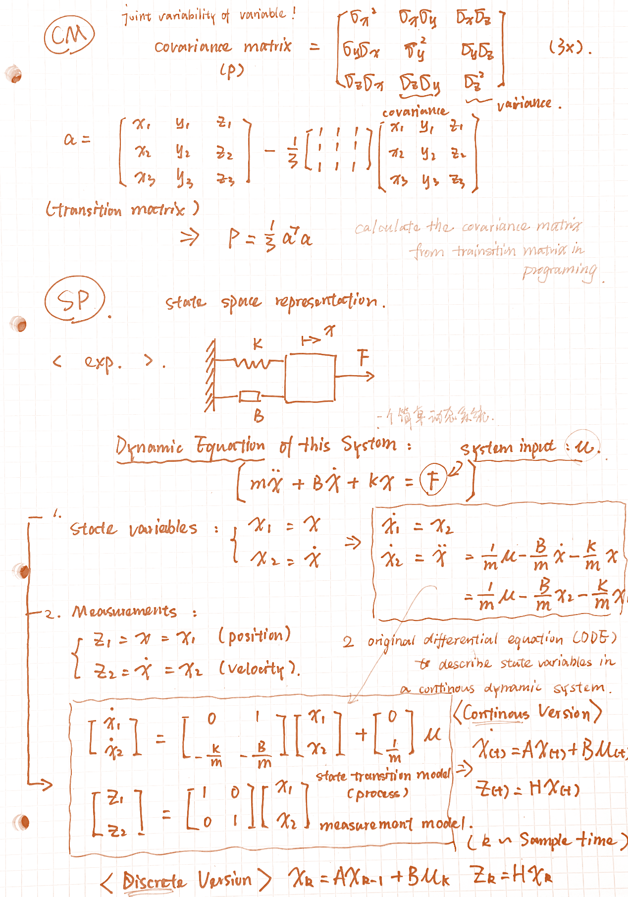
2. Covariance Matrix & State Space
I’m so lazy to type all these down. Fortunately, these are all some very basic content here.
It provides two different versions of dynamic system here, continuous and discrete. Normally the discrete version is just enough. This approach of interpretation on Kalman filter tend to build a recursive data fusion problem in dynamic system. There are also some other ways to understand the Kalman filter, after all it is still a Bayesian filter.
Now we got all we need, from a discrete dynamic system, a uncertain prediction from state transition model and a uncertain measurement from measurement model. Then we just have to conduct the recursive data fusion, what we’ve been talking about all through this page, on the system. OK, then we need a proper Kalman Gain.

